Recently, we visited The Data Science Economy conference in Zagreb. More than 30 speakers covered a lot of real-life use cases, best practices, and future trends in the field of Data Science. We also participated in “Deep Dive into Deep Learning„ workshop held by Leonardo De Marchi, the Lead Data Scientist in Badoo (Badoo is the largest dating site with over 360 million users).
As the Deep Learning is part of our daily work and also the main trend in AI, we decided to share with you some of the insights we learned at this workshop and help you to start your own first deep learning project.
We will go through some of the basic Deep Learning concepts with Keras. Keras is a high-level neural networks API, written in Python and capable of running on top of TensorFlow, CNTK, or Theano. Keras is simple, user-friendly and enables the fast experimentation while modeling. We will examine a real image recognition project and learn how to create a multi-layered neural network. Specifically, how to implement Convolutional Neural Network for image recognition and how to use some more sophisticated techniques like dropouts.
Basic concepts of Deep Learning
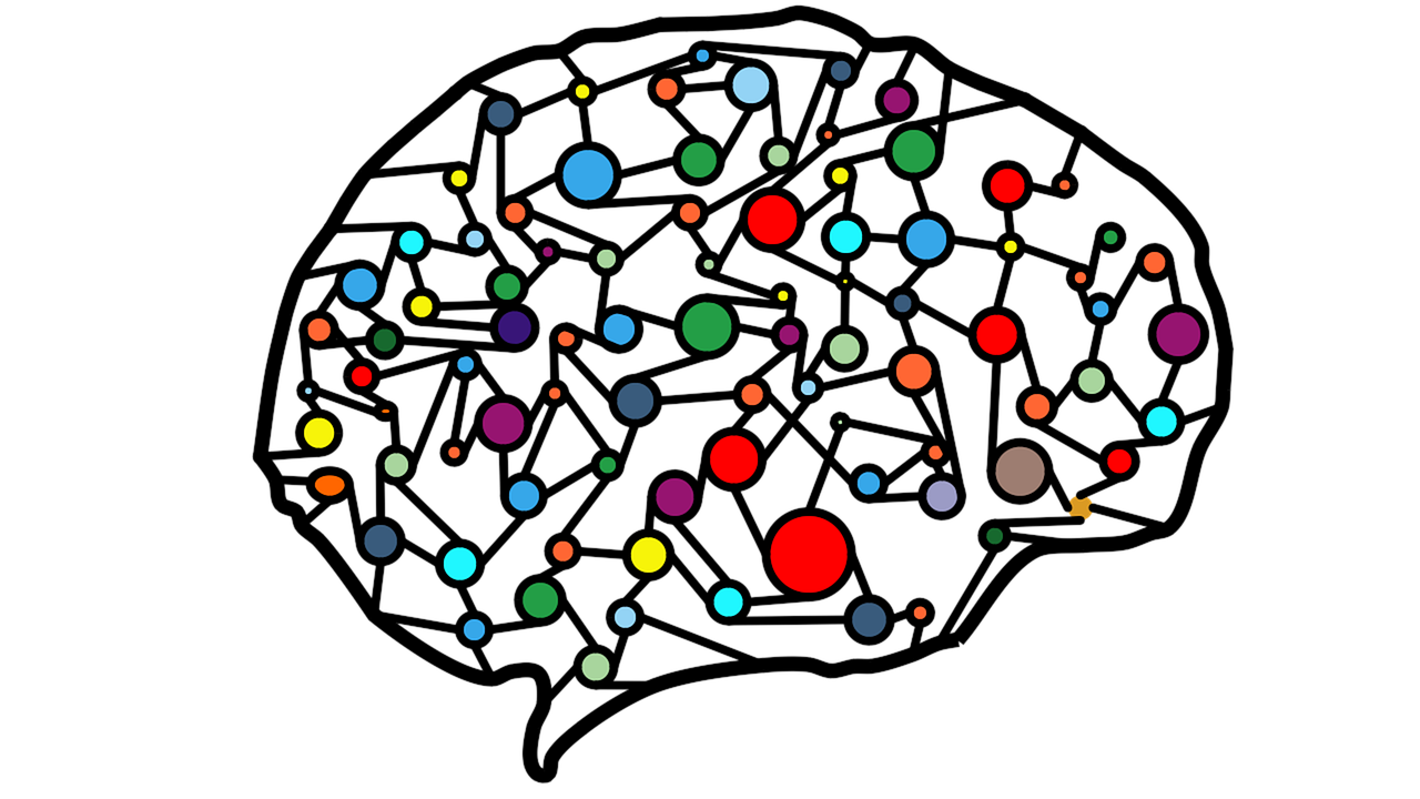
Neural networks are the subset of machine learning techniques. They are modeled to mimic neurons, their connections and interactions in the brain. As signal spreads through the brain, it travels from one neuron to another. Similarly, in a neural network, information spreads layer by layer allowing a computer to learn by itself from the observed data. As neural networks tend to have multiple layers, we often refer to these techniques as Deep Learning.
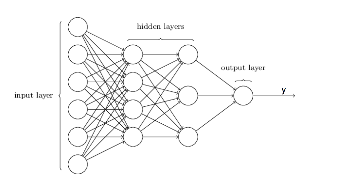
The simplest type of neural network is Feedforward neural network. Its architecture allows information to move only in one direction – forward. From input layer through the “hidden” layers to the output layer, but without any loops along the way. Actually, training any neural network consists of providing input and telling the network what an output should be, while network itself try to figure out the best performing parameters. So, you should always “feed” it with as much data as you can, because it learns with every iteration (i.e. readjusts the parameters). The larger the input the better the results are!
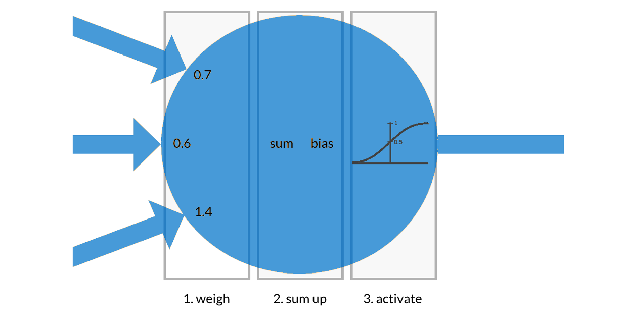
The basic building block of the neural network is an artificial neuron. It processes all inputs and produces an output. All inputs are weighted and summed up with a bias to a single value; which is then turned into an output with an activation/transfer function. Therefore, with every iteration, neural network gradually shifts the weights and biases of all the neurons, in a way that the next iteration output is a bit closer to the known/true output. A measure of the difference between final outputs is called cost function (or loss function) and it should be minimized with learning. We’ll return to these terms in one of our next articles and address the problem of overfitting (model is overfitting when it’s perfect for the training data but crashes for the test data) and teach you how to avoid it.
First example: simple neural network
Let’s start and construct a simple neural network in Keras. We’ll create a neural network that mimics the linear function f(x) = 2*x + 1 . Input for neural network will be 1000 decimal numbers from the interval [1, 2] and outputs will be values of the linear function in those points. We’ll use a sequential model and just stack layers on top of each other, with a marvelous Keras function add(), which allows super fast and super easy neural net construction! You’ll see, it’s pretty simple!
We’ll use only one Dense layer which is an elementary fully connected layer; its activation will be linear (because of the linear function) and parameter initializer will be glorot_uniform (but you can use either one to set starting random weights).
Parameter initializer is a function that creates initial values for model parameters, i.e. it gives them starting values which are updated in every iteration while training.
Output dimension is 1, the same as an input. The final construction step is a model compilation, where you define the loss function and optimizer (i.e. learning method). We’ll use the standard regression loss function: mean square error and an RMSprop optimizer. Note: always use function summary() to get info about created neural network!
Example of model contruction:
import numpy as np
from keras.layers import Dense
from keras.models import Sequential, Model

def linear_f(x):
"""Simple linear function"""
return 2*x+1

x = np.linspace(1,2, num = 1000)

model = Sequential()
model.add(Dense(1, input_dim=1, activation="linear", kernel_initializer="glorot_uniform"))
model.compile(loss='mse', optimizer="rmsprop")
model.summary()
Output:
_________________________________________________________________
Layer (type)                 Output Shape              Param #
=================================================================
dense_2 (Dense)              (None, 1)                 2
=================================================================
Total params: 2
Trainable params: 2
Non-trainable params: 0
_________________________________________________________________
As you can see above, this neural network consists of just one Dense layer and it has only two parameters to configure. We already know that their true values are 2 and 1 (because of the definition of f(x)), but let’s see what neural network will say after training. To train a network, you need an input, output, batch size and number of iterations through the whole dataset (i.e. epochs). Function fit() trains the network while get_weights() gives you the resulting parameters.
If everything is ok, in every iteration you will see the decrease of a loss function.
Example of model training:
model.fit(x, linear_f(x), batch_size=10, epochs=100)
model.get_weights()
Output:
Epoch 1/100
1000/1000 [==============================] - 0s 116us/step - loss: 1.5556e-06
Epoch 2/100
1000/1000 [==============================] - 0s 139us/step - loss: 1.5915e-06
Epoch 3/100
1000/1000 [==============================] - 0s 114us/step - loss: 1.5387e-06
Epoch 4/100
1000/1000 [==============================] - 0s 106us/step - loss: 1.5678e-06
Epoch 5/100
1000/1000 [==============================] - 0s 104us/step - loss: 1.5650e-06
Epoch 6/100
1000/1000 [==============================] - 0s 103us/step - loss: 1.5977e-06
Epoch 7/100
1000/1000 [==============================] - 0s 111us/step - loss: 1.5423e-06
.................................

[array([[2.0006754]], dtype=float32), array([1.0005257], dtype=float32)]
So, the parameters are great! As you can see, the first one is 2.0006754 (a true value is 2) and the second one is 1.0005257 (with true value 1). You can make them even better with more data or more complex neural network (because this architecture is way too basic), but this was also too trivial problem to solve with a neural network.
Second example: Convolutional neural network for image classification
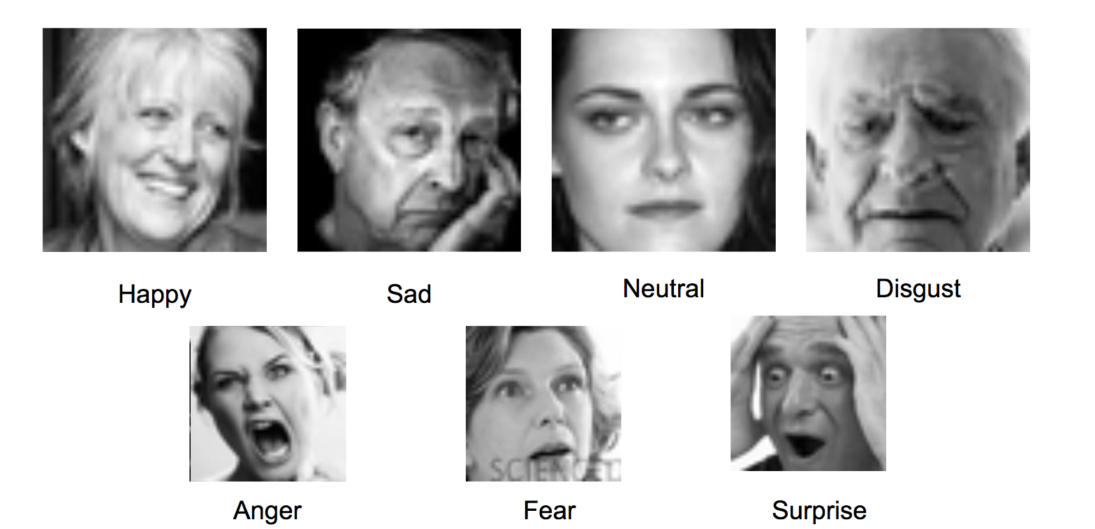
Now, let’s talk about other problem which you may face – image recognition. We are taking the classification of people facial expressions as an example. The observed dataset consists of 28,698 images of shape 48x48 pixels. The task is to categorize each face based on the shown emotion in the facial expression into one of seven categories: angry, disgust, fear, happy, sad, surprise, neutral. The resolution is not great which makes it difficult to gain good accuracy, but overall computing will be faster. So, let’s start!
When working with images, you’ll always use a Convolutional neural network (the form of Feedforward neural net). Every Convolutional network contains three main types of layers: Convolutional layer, Pooling layer, and Fully-Connected layer (exactly as seen in a regular neural network). It arranges the neurons in 3 dimensions: width, height, and depth. The Convolutional layer is specific because it takes as input image presented as a tensor that holds the raw pixel values with dimensions width, height, and with three color channels R, G, B. In our observed dataset, all the pictures are black and white; and because of that one input volume has the size 48x48x1 (the same colored image would be 48x48x3).
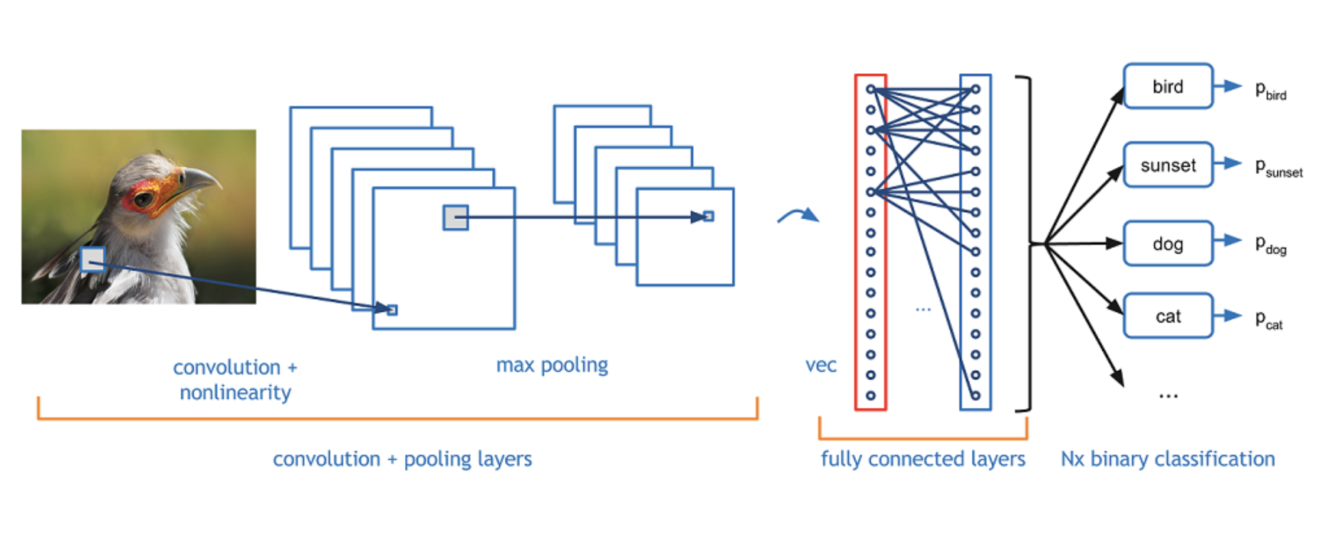
Further, the Pooling layer reduces the spatial size of the image representation, simultaneously reducing the parameter number and the amount of computation. Here, we also added a Dropout layer which randomly drops/forgets a few connections between the neurons in every iteration.
As mentioned before, you can just stack all those layers with function add() like this:
from keras.layers.convolutional import Convolution2D, MaxPooling2D
from keras.layers import Dense, Dropout, Flatten
from keras.models import Sequential

def create_model():
# create model
    model = Sequential()
    model.add(Convolution2D(filters =30, kernel_size= (5, 5), input_shape=(48, 48, 1),padding='same', activation="relu"))
    model.add(MaxPooling2D(pool_size = (2,2), padding='same'))
    model.add(Dropout(0.1))
    model.add(Convolution2D(filters =15, kernel_size= (3, 3), padding='same', activation="relu"))
    model.add(MaxPooling2D(pool_size = (2,2), padding='same'))
    model.add(Dropout(0.2))
    model.add(Flatten())
    model.add(Dense(100, activation="relu"))
    model.add(Dense(50, activation="relu"))
    model.add(Dense(7, activation="softmax"))
return model


my_model = create_model()
my_model.compile(loss='categorical_crossentropy', optimizer='adam', metrics=['accuracy'])
my_model.summary()
Output:
_________________________________________________________________
Layer (type)                 Output Shape              Param #
=================================================================
conv2d_1 (Conv2D)            (None, 48, 48, 30)        780
_________________________________________________________________
max_pooling2d_1 (MaxPooling2 (None, 24, 24, 30)        0
_________________________________________________________________
dropout_1 (Dropout)          (None, 24, 24, 30)        0
_________________________________________________________________
conv2d_2 (Conv2D)            (None, 24, 24, 15)        4065
_________________________________________________________________
max_pooling2d_2 (MaxPooling2 (None, 12, 12, 15)        0
_________________________________________________________________
dropout_2 (Dropout)          (None, 12, 12, 15)        0
_________________________________________________________________
flatten_1 (Flatten)          (None, 2160)              0
_________________________________________________________________
dense_1 (Dense)              (None, 100)               216100
_________________________________________________________________
dense_2 (Dense)              (None, 50)                5050
_________________________________________________________________
dense_3 (Dense)              (None, 7)                 357
=================================================================
Total params: 226,352
Trainable params: 226,352
Non-trainable params: 0
_________________________________________________________________
Let’s now define some parameters and develop a training pipeline. To preprocess images, you can use a combination of ImageDataGenerator() and flow_from_directory() which generate batches of images from input directory. Good practice while training is a use of validation data to estimate accuracy after each iteration.
from keras.preprocessing.image import ImageDataGenerator

img_width, img_height = 48, 48
epochs = 3
batch_size = 50

emotions = {
0: 'Angry',
1: 'Disgust',
2: 'Fear',
3: 'Happy',
4: 'Sad',
5: 'Surprise',
6: 'Neutral'
}

num_classes = len(emotions)
num_train_samples = 28698
num_validation_samples = 3589

train_datagen = ImageDataGenerator(rescale=1. / 255, shear_range=0.2, zoom_range=0.2, horizontal_flip=True)
test_datagen = ImageDataGenerator(rescale=1. / 255)

# Get images from folders
train_generator = train_datagen.flow_from_directory(directory= '../data/raw/Training/', color_mode='grayscale', target_size=(img_width, img_height), batch_size=batch_size, class_mode='categorical', save_to_dir='../data/processed/Training/')
validation_generator = test_datagen.flow_from_directory(directory='../data/raw/PrivateTest/', color_mode='grayscale', target_size=(img_width, img_height), batch_size=batch_size, class_mode='categorical', save_to_dir='../data/raw/PrivateTest/')
Output:
Found 28698 images belonging to 7 classes.
Found 3589 images belonging to 7 classes.
To train a model, we’ll just use fit_generator() and validate the result after every epoch:
my_model.fit_generator(train_generator, steps_per_epoch=num_train_samples // batch_size, epochs=epochs, validation_data=validation_generator, validation_steps=num_validation_samples // batch_size)
Output:
Epoch 1/3
573/573 [==============================] - 114s 199ms/step - loss: 1.7275 - acc: 0.3048 - val_loss: 1.6134 - val_acc: 0.3738
Epoch 2/3
573/573 [==============================] - 102s 179ms/step - loss: 1.5892 - acc: 0.3797 - val_loss: 1.4978 - val_acc: 0.4200
Epoch 3/3
573/573 [==============================] - 108s 189ms/step - loss: 1.5270 - acc: 0.4047 - val_loss: 1.4461 - val_acc: 0.4341
Final prediction results are returned in a form of a vector which values represent the percentages of certainty that image belongs to each class. We’ll take the next picture to test our classifier.

Predictions are generated with a predict_generator() function used on the model:
demo_generator = test_datagen.flow_from_directory(directory='../data/demo/', color_mode='grayscale', target_size=(img_width, img_height), batch_size=1, class_mode='categorical', save_to_dir='../data/raw/PrivateTest/')

predictions = my_model.predict_generator(demo_generator, steps=1)

for i, prediction in zip(emotions, predictions[0]):
    print('{emotion: <8} - {score:5.2f}%'.format(emotion=emotions[i], score=prediction*100))
Output:
Found 1 images belonging to 1 classes.
Angry    -  0.82%
Disgust  -  0.06%
Fear     -  1.74%
Happy    - 91.68%
Sad      -  3.29%
Surprise -  1.27%
Neutral  -  1.14%
In our testing example, you can see that neural network classifies the upper person as happy with the certainty of 91%. It also finds some features specific for a sad person (maybe eyes looks bit sad) but the overall result is great. The accuracy could be better with more data or bit different network, but you have to take into the account that all pictures have a really small resolution.
We hope our examples will be useful for everyone who wants to make a first dive into deep learning. Neural networks are currently the number one machine learning algorithms in the field of image classification, speech recognition, self-driving vehicles, machine translation, question-answering and dialogue systems. Their training demands a huge amount of data and large computational power, but their advantages are remarkable! Their main disadvantage is a “black box” learning - it is impossible to interpret connections between the input and the output. Currently, no one knows the exact structure of functions approximated by neural networks, but they work! And they are the future of technology!
In our next articles, we will share some tips and tricks for working with neural networks and more complex examples of using deep learning in practice.

